Topological insulators
25 Jun 2025This article is based on my seminar report1 on topological insulators, prepared at Leiden University. The work gives a pedagogical overview of the topological description of band insulators, with a primary focus on the Kane–Mele model of graphene and the emergence of the ℤ₂ topological phase. Along the way, I introduce the necessary mathematical tools like vector bundles and their topological invariants and illustrate them on the Haldane and Kane–Mele models.
Introduction
Topological insulators are phases of matter which cannot be distinguished from ordinary insulators by the usual Landau picture based on spontaneous symmetry breaking and local order parameters. Instead, what matters is the global structure of the electronic bands. Roughly speaking, the valence bands of an insulator can carry non-trivial topology, and this topology cannot be changed continuously unless the energy gap closes.
One of the main reasons this topic became so important is that non-trivial bulk topology is accompanied by robust conducting states at the boundary. These edge or surface states are not just a mathematical curiosity. They are probably the most interesting feature of topological phases from the point of view of applications, because they can be protected against certain kinds of disorder and backscattering. The subject is therefore interesting not only conceptually, but also technologically. In the broader family of topological phases, related ideas also appear in the search for Majorana quasiparticles and in proposals for topological quantum computing, which promises error protection already at the hardware level. Microsoft is one of the companies actively pursuing this direction, as illustrated for example by the recent Nature paper6. At the same time, I think it is important to keep some scepticism here. There is a lot of excitement around these applications, but it is still not clear how close we are to fully practical devices built on these principles.
The modern study of topological insulators was shaped in large part by the two seminal papers of Kane and Mele23, which showed that graphene with spin–orbit coupling provides a natural setting for a new kind of time-reversal invariant topological phase. Kane also later wrote a very nice pedagogical introduction to the topic, which I found especially useful for building intuition.4 Although the original Kane–Mele model is not realized in actual graphene because the spin–orbit coupling there is too weak, closely related physics was later realized experimentally in HgTe quantum wells.5
From bands to topology
To understand where topology enters band theory, it is useful to think of the eigenstates of the Bloch Hamiltonian as varying over momentum space. In a crystal, Bloch’s theorem tells us that single-particle states can be labelled by crystal momentum \(\mathbf{k}\), which lives in the Brillouin zone. In two dimensions, the Brillouin zone is topologically a torus \(\mathbb{T}^2\).
At each momentum \(\mathbf{k}\), the Bloch Hamiltonian has a finite-dimensional Hilbert space of eigenstates. If we focus on the states below the Fermi energy, that is the valence bands, these states form what is called the valence Bloch bundle over the Brillouin zone. This is the object whose topology we study.
One can think of a vector bundle very roughly as assigning a vector space to each point of some base space. Here the base space is the Brillouin zone and the fibres are the spaces of valence states. A trivial bundle is just a simple product, where one can choose the states continuously everywhere in momentum space without running into any obstruction. A non-trivial bundle is twisted in a global way.
An intuitive picture is the difference between a cylinder and a Möbius strip. Locally they both look simple, but globally the Möbius strip contains a twist that cannot be removed continuously.
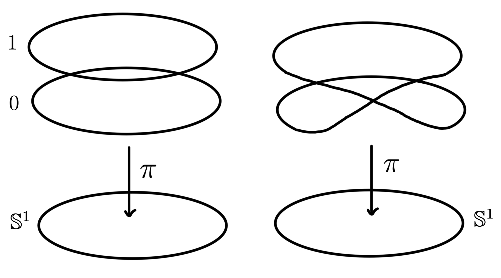
This picture should not be taken too literally, but it captures the essential idea. In band theory, non-trivial topology means that the valence states cannot be globally chosen in a completely smooth and symmetry-compatible way over the whole Brillouin zone. As long as the gap between valence and conduction bands stays open, this topology cannot change under adiabatic deformations of the Hamiltonian.
Graphene
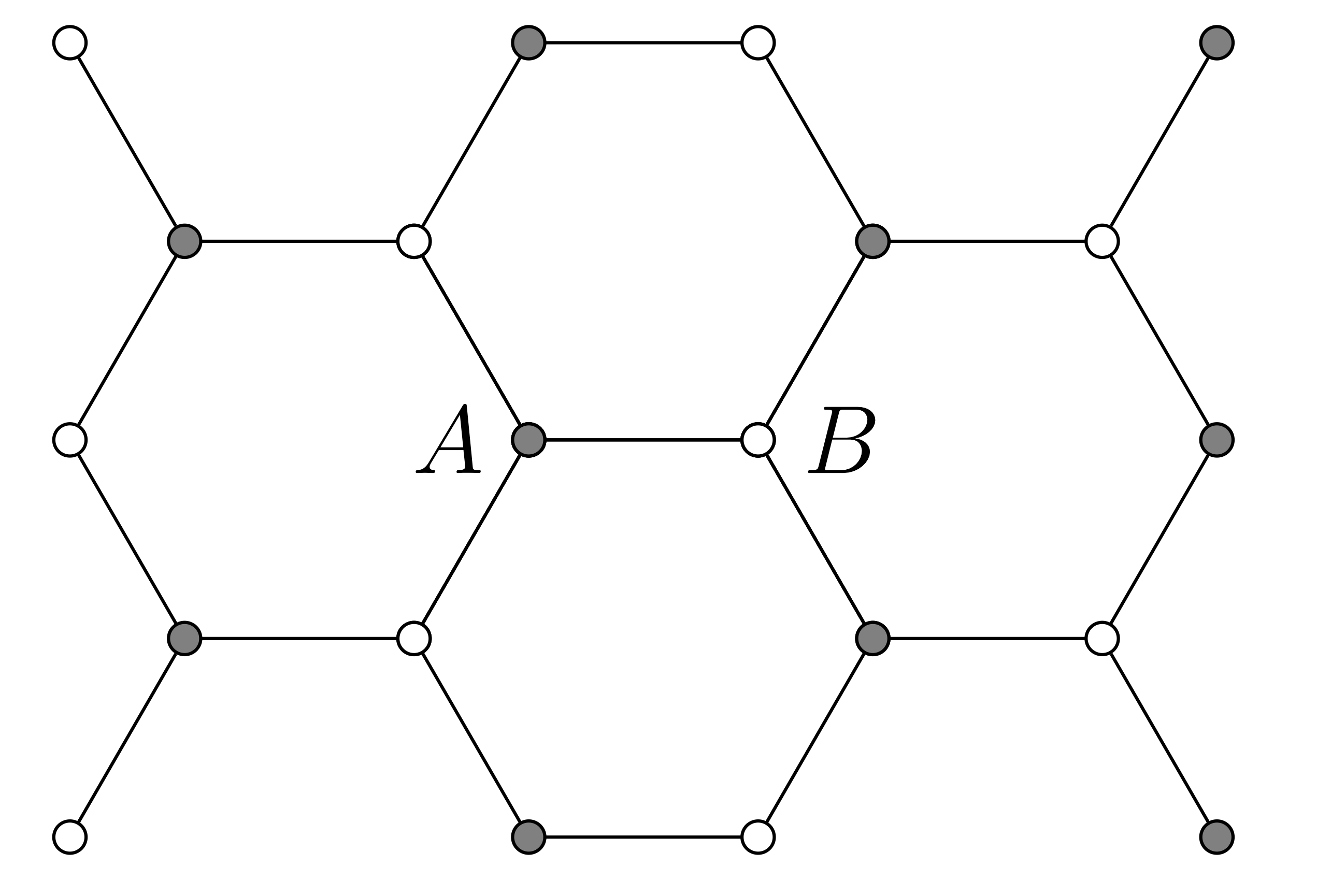
The basic arena for both the Haldane and Kane–Mele models is graphene. Graphene has a honeycomb lattice, which is not itself a Bravais lattice but can be viewed as two interpenetrating triangular sublattices, usually denoted \(A\) and \(B\).
Because of this two-sublattice structure, the low-energy electronic states naturally come with a two-component structure. Near the special points \(\pm\mathbf{K}\) in the Brillouin zone one may write the momentum as \(\mathbf{k} = \pm \mathbf{K} + \mathbf{q}\), where \(\mathbf{q}\) measures the deviation from the Dirac points. In this regime the effective Hamiltonian takes the form of a two-dimensional Dirac Hamiltonian
\[H_{\mathrm{eff}}(\mathbf q) = v_F \,\mathbf q \cdot \boldsymbol{\sigma} + \Delta \,\sigma_z ,\]| where \(\mathbf q \cdot \boldsymbol{\sigma} =\mp q_x \sigma_x + q_y \sigma_y\), \(v_F\) is the Fermi velocity and the Pauli matrices act on the sublattice degree of freedom. The parameter \(\Delta\) controls the gap in the spectrum (the full band gap is $$2 | \Delta | $$). |
In this low-energy description the topological properties are controlled precisely by how this gap parameter behaves at the two valleys \(\pm\mathbf{K}\). This is one of the reasons the Dirac picture is so useful: it makes the origin of the topology very transparent. What matters is not every microscopic detail of the lattice model, but the structure of the gaps in the effective theory near the points where the bands would otherwise touch.
Chern insulators and the Haldane model
Before turning to the Kane–Mele model, it is useful to look at the simpler case of a Chern insulator. Here the relevant topological invariant is the Chern number.
To see where it comes from, recall that the valence states of an insulator form the valence Bloch bundle over the Brillouin zone \(\mathbb{T}^2\). A natural gauge freedom appears because the overall phase of a single-particle wave function is not observable. This means that the bundle carries a \(U(1)\) gauge symmetry, very much like in ordinary gauge theory.
Once such a gauge freedom is present, it is natural to introduce a connection on the bundle. In condensed matter physics one usually works with the Berry connection, which is the connection associated with the adiabatic variation of the Bloch Hamiltonian with momentum \(k\). But since we are computing a topological invariant one may choose completely arbitrary connection.
Every connection \(A\) has an associated curvature two-form
\[F = dA .\]The topology of the bundle can then be characterized using Chern–Weil theory, which associates topological invariants to curvature forms. For a single valence band the resulting invariant is the first Chern number
\[c_1 = \frac{1}{2\pi}\int_{T^2} F ,\]and the remarkable fact is that this quantity is always an integer, which ultimately follows from the underlying algebraic topology of the bundle.
Physically, the Chern number is important because of the so called TKNN relation, which connects it directly to Hall conductivity:
\[\sigma_{xy} = \frac{e^2}{h}\, c_1 .\]So in this case topology is not just abstract mathematics. It becomes directly observable as a quantized transport coefficient.
A famous theoretical model realizing this physics on the graphene lattice is Haldane’s model. It describes a system with no net magnetic flux through the unit cell, but with a pattern of complex next-nearest-neighbour hopping terms that still breaks time-reversal symmetry. In this way one obtains a quantized Hall effect without an overall external magnetic field, the so-called anomalous quantum Hall effect.
In the low-energy description discussed in the previous section, the Hamiltonian still has the Dirac form (see the equation above). The effect of the Haldane terms is simply to generate a valley-dependent gap parameter \(\Delta = \lambda_v \pm 3\sqrt{3}\,t_2 \sin\phi\), where the sign again depends on around which Dirac point one expands.
As also already mentioned the topology is determined by the behaviour of \(\Delta\) at the Dirac points, specifically the Chern number can be expressed as
\[c_1 = \frac{1}{2}\left[\operatorname{sgn}(\Delta(\mathbf{K}))-\operatorname{sgn}(\Delta(-\mathbf{K}))\right].\]One sees that, if the gaps at the two valleys have opposite signs, the system is in a topological phase with \(c_1=\pm1\). If the signs are the same, the contributions cancel and the phase is topologically trivial.
This model is conceptually very important even though it is not naturally realized in graphene itself. It provides the cleanest prototype of a Chern insulator and, more importantly for us, it serves as the building block for understanding the Kane–Mele model23.
Kane–Mele model and the quantum spin Hall effect
The Kane–Mele model extends the graphene Dirac picture by including the electron spin. The Hamiltonian can be written as two blocks corresponding to the two spin sectors plus a spin mixing term
\[H_{KM}(\mathbf{k}) = \begin{pmatrix} H_H^{\uparrow}(\mathbf{k}) & 0 \\ 0 & H_H^{\downarrow}(\mathbf{k}) \end{pmatrix} + H_R(\mathbf{k}) \,,\]where \(H_H^{\uparrow}\) and \(H_H^{\downarrow}\) are Haldane Hamiltonians with opposite effective fluxes. In particular they correspond to the Haldane model with parameters \(t_2 = \lambda_{so}\) and \(\phi = \pm \frac{\pi}{2}\).
For sufficiently strong intrinsic spin–orbit coupling \(\lambda_{so}\) these two Haldane models therefore lie in topological phases with Chern numbers \(c_1^{\uparrow}=+1\) and \(c_1^{\downarrow}=-1\).
This structure originates from spin–orbit coupling, which couples the electron spin to its motion in the lattice potential. In graphene the intrinsic spin–orbit interaction effectively generates opposite Haldane-type terms for the two spin sectors.
In the low-energy theory near the Dirac points the intrinsic spin–orbit interaction takes the simple form
\[H_{so}^{\mathrm{eff}} = \pm \Delta_{so}\, \sigma^z \otimes \sigma^z \, , \qquad \Delta_{so} := 3\sqrt{3}\,\lambda_{so}.\]The Kane–Mele model can also contain a Rashba spin–orbit term, which mixes the spin sectors. In the effective theory it reads
\[H_R^{\mathrm{eff}}(\mathbf{k}) = \Delta_R(\pm \sigma^y \otimes \sigma^x - \sigma^x \otimes \sigma^y)\,, \qquad \Delta_R := \frac{3}{2}\lambda_R .\]Unlike the intrinsic spin–orbit term, this interaction does not preserve the spin \(z\)-component and therefore prevents us from viewing the model simply as two independent Haldane systems. In the regime where the Rashba coupling is small, however, the two spin sectors remain approximately decoupled.
In that simplified regime the model effectively splits into two copies of Haldane’s model: one for spin up and one for spin down. These two copies are related by time-reversal symmetry, so their Chern numbers are opposite \(c_1^\uparrow = -c_1^\downarrow\). As a result the total charge Hall conductivity vanishes, which is exactly what one expects in a time-reversal invariant system. However, one can still define a spin Hall conductivity. If we denote it by
\[\sigma_{xy}^s := \frac{\hbar}{e}\, \frac{\sigma_{xy}^{\uparrow}-\sigma_{xy}^{\downarrow}}{2},\]then using the TKNN relation one finds
\[\sigma_{xy}^s = \frac{e}{2\pi}\, n_s ,\]where \(n_s = \frac{c_1^{\uparrow}-c_1^{\downarrow}}{2}\).
Thus the spin Hall response is quantized. This is the quantum spin Hall (QSH) phase discussed in the original Kane–Mele paper.2
From this point of view the \(\mathbb{Z}_2\) invariant admits a very intuitive interpretation. One may define \(z_2 \equiv n_s \pmod{2}\).
If the two spin sectors carry opposite Chern numbers, then \(z_2=1\) and the phase is topologically non-trivial. If they are both trivial, then \(z_2=0\). In this regime one may therefore think of the quantum spin Hall phase simply as two time-reversed Haldane models glued together.
This is not yet the full story. In the more general Kane–Mele model the Rashba interaction mixes the spin sectors and the separate Chern numbers are no longer well defined. Nevertheless the non-trivial \(\mathbb{Z}_2\) phase survives beyond this simplified regime. For the purposes of this post I kept the discussion at the level of the quantum spin Hall regime, but more about the treatment of the general case can be found in the work itself.1
Edge states and why they matter
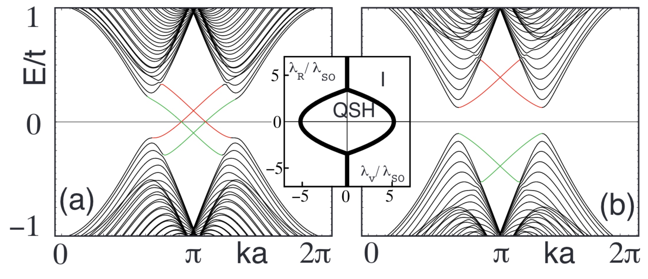
The most striking consequence of non-trivial bulk topology is the existence of boundary modes. In a Chern insulator, these are chiral edge states: they move only in one direction along the boundary. In the quantum spin Hall regime of the Kane–Mele model, they become helical edge states: opposite directions of motion are tied to opposite spin sectors.
This edge physics is in many ways the most important part of the story. At the interface between a topological and a trivial phase, the bulk gap must close, and this produces gapless states localized near the boundary. In the topological regime these edge states cross the bulk gap and connect valence and conduction bands. In the trivial regime they do not.
In the helical case, a right-moving edge mode and a left-moving edge mode form a time-reversal pair. Because of this, elastic backscattering from non-magnetic disorder is strongly suppressed. To scatter backwards, the electron would have to flip into its time-reversed partner, and time-reversal symmetry prevents generic perturbations of this kind from opening a gap. This robustness is the main reason edge states are so interesting for transport and for applications.
Of course, one should not oversell this. Real materials are never ideal, interactions can matter, disorder is not always harmless, and practical device design is much harder than the clean theoretical picture suggests. Still, the general mechanism is extremely robust conceptually: bulk topology enforces protected boundary states, and those boundary states can carry current in an unusually stable way.
This is one of the central lessons of topological condensed matter. The important physics is not only in the local form of the Hamiltonian, but in its global topological structure. And once that topology is non-trivial, the boundary has no choice but to respond.
Why I find this topic interesting
What I find especially attractive about this subject is how naturally it connects abstract mathematics with concrete physics. Objects like vector bundles, Berry curvature and topological invariants are not added artificially. They arise quite directly once one starts taking the global structure of Bloch states seriously.
This topic is a nice example of a broader theme that appears again and again in theoretical physics: ideas that originally look abstract or formal often end up describing very real phenomena. In this case, concepts from geometry and topology became part of the language used to understand actual quantum materials, and possibly future technologies built from them.
1: J. Masák, Topological insulators, Seminar Report, Science faculty, Leiden university (2025), PDF.
2: C. L. Kane, E. J. Mele, Quantum Spin Hall Effect in Graphene, Phys. Rev. Lett. 95 (2005) 226801, doi:10.1103/PhysRevLett.95.226801.
3: C. L. Kane, E. J. Mele, $\mathbb{Z}_2$ Topological Order and the Quantum Spin Hall Effect, Phys. Rev. Lett. 95 (2005) 146802, doi:10.1103/PhysRevLett.95.146802.
4: C. L. Kane, Topological Band Theory and the $\mathbb{Z}_2$ Invariant, in Topological Insulators, Contemporary Concepts of Condensed Matter Science 6, Elsevier (2013) 3–34, doi:10.1016/B978-0-444-63314-9.00001-9.
5: M. König, S. Wiedmann, C. Brüne, A. Roth, H. Buhmann, L. W. Molenkamp, X.-L. Qi, S.-C. Zhang, Quantum Spin Hall Insulator State in HgTe Quantum Wells, Science 318 (2007) 766–770, doi:10.1126/science.1148047.
6: M. Aghaee, A. Alcaraz Ramirez, Z. Alam, et al., Interferometric single-shot parity measurement in InAs–Al hybrid devices, Nature 638 (2025), doi:10.1038/s41586-024-08445-2.