ϕ

• home
• about
• articles
• contact

Argon gas simulation

20 Mar 2025

This article is based on a computational physics project¹ carried out at Leiden University. In the project, the motion of a relatively small number of Argon atoms was simulated using simple Newtonian dynamics with the Lennard–Jones potential, integrated using the Verlet algorithm with periodic boundary conditions. The aim was to see how this microscopic model reproduces the three phases of matter and to study their basic properties. Here I give a short conceptual exposition of the work. The simulation code used in the project is available on GitHub.

Molecular dynamics and Argon

Molecular dynamics aims to follow the motion of many interacting particles by numerically solving their equations of motion. Early simulations of this kind already demonstrated phase behaviour in simple interacting systems². In this approach each atom is treated as a classical particle and its trajectory is obtained by integrating Newton’s equations. Even a relatively simple interaction model can already reproduce many properties of real materials.

In the simulation each particle obeys Newton’s second law

\[m \frac{d^2 \mathbf{x}}{dt^2} = \mathbf{F}(\mathbf{x}) = - \nabla U(\mathbf{x}) .\]

If the interaction potential is a sum of pair interactions, the force on particle \(\alpha\) can be written as

\[\mathbf{F}_\alpha = - \sum_{\beta \neq \alpha} \nabla U(\mathbf{x}_\alpha - \mathbf{x}_\beta).\]

Once the potential is specified, the task of the simulation is therefore to repeatedly compute the forces and update the particle positions.

Lennard–Jones potential

For Argon atoms the interaction can be modeled by the Lennard–Jones two-particle potential

\[U(r) = 4\varepsilon \left[\left(\frac{\sigma}{r}\right)^{12} - \left(\frac{\sigma}{r}\right)^6 \right].\]

Here \(r\) is the distance between the two particles, while \(\varepsilon\) and \(\sigma\) set the energy and length scales of the interaction.

The \(r^{-12}\) term produces a strong short-range repulsion, preventing atoms from occupying the same position. The \(r^{-6}\) term represents an attractive van der Waals interaction. Together they create a preferred separation between atoms, corresponding to the minimum of the potential at \(r_{\min} = 2^{1/6}\sigma\).

This preferred distance later appears as the first peak in the pair-correlation function.

Numerical integration

To evolve the system in time we integrate the equations of motion numerically. In this project the velocity Verlet algorithm⁴ was used because it is simple and stable for long simulations.

The positions are updated according to

\[\mathbf{x}(t+h)=\mathbf{x}(t)+h\mathbf{v}(t)+\frac{h^2}{2m}\mathbf{F}(\mathbf{x}(t))+\mathcal{O}(h^3)\,.\]

The velocity update uses the forces at the beginning and end of the step

\[\mathbf{v}(t+h)=\mathbf{v}(t)+\frac{h}{2m}(\mathbf{F}(\mathbf{x}(t+h))+\mathbf{F}(\mathbf{x}(t)))+\mathcal{O}(h^3)\,.\]

In the continuous equations of motion the total energy is conserved. This follows from the invariance of the physical laws under time translations, as expressed by Noether’s theorem. When the equations are discretised this symmetry is generally broken. For example, a simple Euler integration scheme treats the forward and backward directions in time differently and typically leads to a gradual drift of the energy.

The Verlet algorithm improves this behaviour by making the update rule explicitly symmetric under the transformation \(t \to -t\). Although the energy is not exactly conserved, it typically oscillates around the correct value instead of drifting systematically. This makes the method particularly well suited for long molecular dynamics simulations.

Periodic boundary conditions and the minimum image convention

The number of particles in a simulation is necessarily limited. To mimic a much larger system we use periodic boundary conditions.

Particles move inside a cubic box of side length \(L\). Whenever a particle leaves the box through one side it re-enters through the opposite side. One can think of the simulation box as being surrounded by infinitely many copies of itself. This removes artificial boundary effects and makes the system behave more like a small piece of bulk matter.

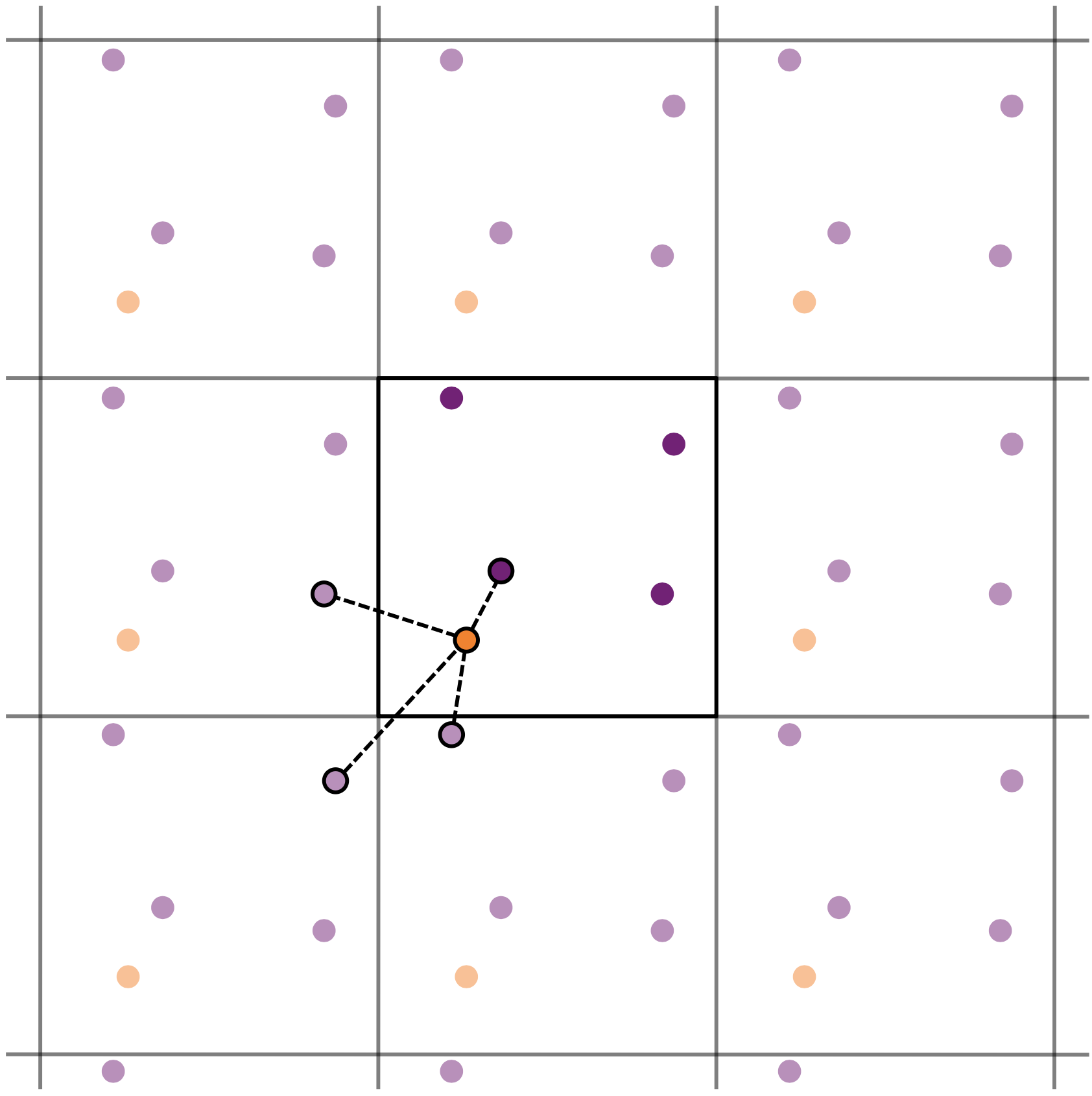
Under periodic boundary conditions each particle has infinitely many periodic images. When computing forces we therefore need a rule that determines which image interacts with a given particle. The minimum image convention states that particles interact only with the nearest periodic image as illustrated in the image below.

Formally the relative position between two particles can be written as

\[r_{\alpha\beta} = \min_{k,l,m \in \{-1,0,1\}} \left| \mathbf{x}_\alpha - \mathbf{x}_\beta + (k,l,m)\,L \right|.\]

Because the simulation box is orthogonal, the shortest displacement can be obtained by shifting each coordinate difference into the interval \((-L/2, L/2)\). In practice this can be implemented using the modulo operation

\[\Delta x = (x_\alpha - x_\beta + L/2)\ \mathrm{mod}\ L - L/2 ,\]

and similarly for \(\Delta y\) and \(\Delta z\). The displacement vector is then \(\mathbf{r}_{\alpha\beta} = (\Delta x, \Delta y, \Delta z)\).

Initial configuration and equilibration

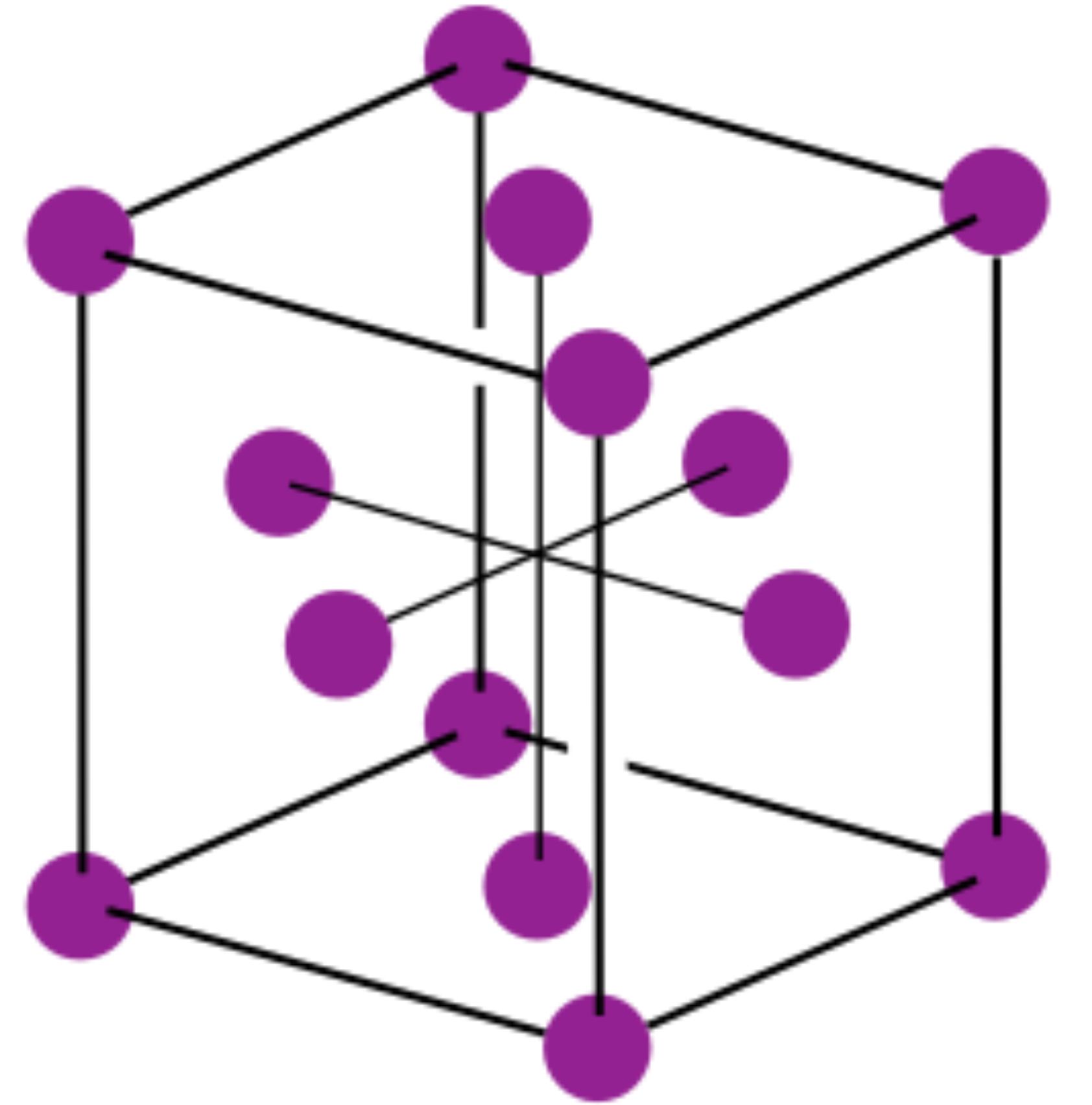
To avoid extremely large forces the atoms are initially placed on a face-centered cubic lattice, which is the crystal structure into which Argon solidifies. The initial separation between atoms is chosen to correspond to the observed lattice spacing of solid Argon. In practice such structural parameters can be obtained from experiment or from electronic structure calculations. The unit cell of the face-centered cubic lattice is illustrated in the image below.

Initial velocities are chosen from a Maxwell distribution corresponding to the desired temperature. The system is then evolved for a number of steps while rescaling the velocities so that the kinetic energy approaches the expected value

\[E_{\mathrm{kin}} = (N-1)\frac{3}{2}k_B T .\]

This equilibration stage allows the system to settle into a representative state before measurements are taken.

Pair-correlation function

One of the most informative observables is the pair-correlation function, which was famously analysed in Rahman’s early molecular dynamics simulation of liquid Argon³. In the project some of the results reported in that work were also reproduced numerically, allowing for a direct comparison with the classical simulation of liquid Argon.

In the simulation the pair-correlation function is defined as

\[g(r) = \frac{2V}{N(N-1)} \frac{\langle n(r)\rangle}{4\pi r^2 \Delta r}.\]

Here \(n(r)\) denotes the number of particles found at a distance between \(r\) and \(r+\Delta r\) from a chosen reference particle.

Roughly speaking, \(g(r)\) measures how likely it is to find another atom at distance \(r\) compared to a completely uniform distribution. The structure of this function therefore reveals the spatial organization of the system.

Gas phase

In the gas phase the particles move freely and there is little spatial structure. The trajectories in the animation below show that the atoms travel through the simulation box with frequent collisions but without forming any persistent structure.

The corresponding pair-correlation function is shown in the plot below.

It is nearly flat with \(g(r) \approx 1\) except at very small distances where the strong repulsive core of the Lennard–Jones potential suppresses close approaches between atoms.

Liquid phase

In the liquid phase the atoms still move throughout the system but remain correlated with their neighbours. This can already be seen in the trajectories below, where particles continuously change their neighbours while remaining part of a relatively dense local environment.

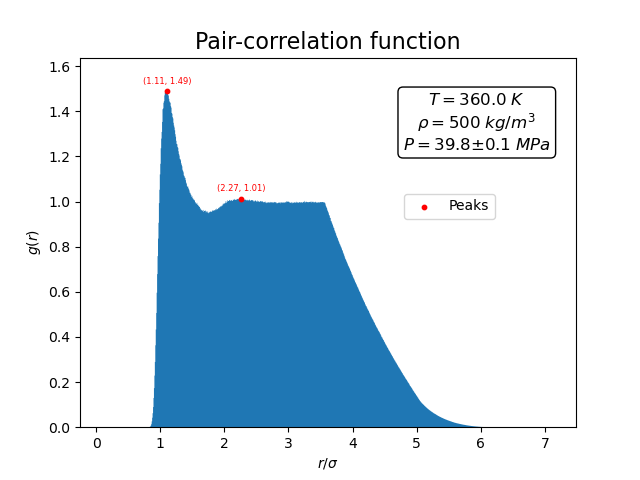
The pair-correlation function shown below reflects this short-range order.

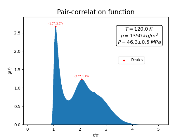
A pronounced first peak appears near the preferred interatomic separation, together with weaker oscillations at larger distances. These peaks indicate that atoms tend to arrange themselves in shells around each other, even though the long-range order of a crystal is absent.

Solid phase

In the solid phase atoms remain localized near lattice sites and only oscillate around their equilibrium positions. This behaviour can be seen clearly in the trajectories below.

The corresponding pair-correlation function shows a series of sharp peaks.

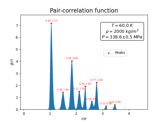
These peaks correspond to the well-defined distances between atoms in the underlying crystal lattice. In contrast to the liquid case, the peaks remain pronounced even at larger distances, reflecting the long-range order characteristic of the solid phase.

Conclusion

Although the model is very simple, it already reproduces the qualitative behaviour of gases, liquids and solids. Even with a relatively small number of particles the characteristic differences between these phases become visible in the particle trajectories and in the pair-correlation function.

This illustrates a central idea of statistical physics: macroscopic properties of matter can often be understood as emerging from simple microscopic dynamics.

---

1: J. Masák, E. Tõkke, Computational Physics Project 1: Molecular Dynamics Simulation of Argon Atoms, Course Project Report, Science faculty, Leiden university (2025), PDF.

2: B. J. Alder, T. E. Wainwright, Phase Transition for a Hard Sphere System, J. Chem. Phys. 27 (1957) 1208, doi:10.1063/1.1743957.

3: A. Rahman, Correlations in the Motion of Atoms in Liquid Argon, Phys. Rev. 136 (1964) A405, doi:10.1103/PhysRev.136.A405.

4: L. Verlet, Computer “Experiments” on Classical Fluids. I. Thermodynamical Properties of Lennard-Jones Molecules, Phys. Rev. 159 (1967) 98, doi:10.1103/PhysRev.159.98.