XY model simulation
05 May 2025This article is based on a computational physics project1 carried out at Leiden University. In the project, the two-dimensional XY model was simulated on a square lattice using the Metropolis Monte Carlo algorithm with periodic boundary conditions. The goal was to explore the thermodynamic behaviour of the model and to reproduce the Kosterlitz–Thouless phase transition. Here I give a short conceptual overview of the work. The simulation code used in the project is available on GitHub.
Introduction
The XY model imagines a two-dimensional lattice \(\Lambda\) of sites \(i \in \Lambda\), at each of which there is a vector \(\mathbf{s}_i \in \mathbb{S}^1\) of unit length. This can be viewed as a generalisation of the Ising model because \(\mathbb{S}^0 = \{-1,1\}\). Each configuration is then represented by a set of spins \(\{\mathbf{s}_i\}_{i \in \Lambda}\) or, equivalently, through the parametrisation \(\mathbf{s}_i = (\cos \theta_i, \sin \theta_i)\), with \(\theta_i \in [-\pi,\pi)\), by a set of angles \(\Theta = \{\theta_i\}_{i \in \Lambda}\), which is the representation I will use most often.
The Hamiltonian used in the simulations can be written as a sum of two parts,
\[H[\Theta] = H_0[\Theta] + H_h[\Theta].\]The first term
\[H_0[\Theta] = -J \sum_{\langle i,j \rangle} \mathbf{s}_i \cdot \mathbf{s}_j = -J \sum_{\langle i,j \rangle} \cos(\theta_i-\theta_j)\]describes the interaction between nearest neighbours and favours alignment of neighbouring spins. The second term
\[H_h[\Theta] = -\mathbf{h}\cdot \sum_{i \in \Lambda} \mathbf{s}_i = -h \sum_{i \in \Lambda} \cos \theta_i\]represents the coupling to an external magnetic field of magnitude \(h = \lVert \mathbf{h} \rVert\) pointing in the \(x\) direction.
The key property of the model lies in the symmetry of the interaction term \(H_0\). Because it depends only on angle differences, it has the symmetry
\[H_0[\Theta] = H_0[\Theta+\Delta\theta], \qquad \Delta\theta \in [-\pi,\pi),\]which is a global \(U(1)\) symmetry. This is probably the most important difference from the Ising model, which also has a global symmetry, but only a discrete \(\mathbb Z_2\) symmetry. Because of this continuous symmetry, we have the Mermin–Wagner theorem2, which states that in a system with such local interactions, continuous symmetries cannot be spontaneously broken at finite temperature when the spatial dimension is \(\leq 2\). This means that in the thermodynamic limit the system cannot develop a non-zero mean magnetisation serving as an ordinary order parameter.
The physical mechanism behind this is the existence of long-wavelength spin waves. Deviations from order can then be quantified by the momentum-space integral
\[\int \frac{d^2k}{k^2}.\]If the lattice is \(N\times N\), this integral scales as \(\ln N\) and therefore diverges in the thermodynamic limit. Since in the simulation the lattice is finite, the divergence is only logarithmic, and as we will see, the system can still look magnetised at low temperatures. This is one of the reasons finite-size effects are important in the XY model.
The absence of spontaneous magnetisation also means that the system does not fit the standard Landau picture of phase transitions based on a local order parameter. Nevertheless, the two-dimensional XY model still exhibits a phase transition, first described by Kosterlitz and Thouless3. It is a topological phase transition, associated with the behaviour of vortices. In our work, we also studied the effect of an external magnetic field. Since the term \(H_h\) explicitly breaks the global \(U(1)\) symmetry, one expects the Kosterlitz–Thouless transition to disappear once the field is switched on. This is indeed what the simulation suggests.
Monte Carlo integration and the Metropolis algorithm
The Monte Carlo method is a powerful approach for studying the properties of a system at equilibrium when we are not interested in its dynamics and need to calculate high-dimensional integrals. In statistical physics, we typically have to evaluate integrals of the form
\[\langle A \rangle = \int_M \mathcal{D}\Theta \, \frac{e^{-\beta H[\Theta]}}{Z} \, A[\Theta], \qquad Z = \int_M \mathcal{D}\Theta \, e^{-\beta H[\Theta]},\]with \(\mathcal{D}\Theta = \prod_{i\in\Lambda} d\theta_i\) and \(M = [-\pi,\pi)^{N^2}\), which can be thought of as the configuration space of the system. We therefore have a very high-dimensional integral, and additional complexity arises from the fact that the function \(A[\Theta]e^{-\beta H[\Theta]}\) is usually very sharply peaked. This requires that we do not sample over the configuration space with the uniform distribution, as the simplest Monte Carlo method does, but instead use importance sampling.
Importance sampling can be implemented by means of the Metropolis algorithm4. This algorithm is also convenient because it assumes that we know the target distribution only up to a normalisation factor. This is exactly the case with the Boltzmann distribution
\[\pi[\Theta(t)] = \frac{e^{-\beta H[\Theta(t)]}}{Z},\]because we do not know the partition function \(Z\).
The Metropolis algorithm can be understood using the concept of a Markov chain: a set of random states \(\Theta(t)\), where the probability of \(\Theta(t+1)\) depends only on \(\Theta(t)\). A Markov chain is fully described by transition probabilities \(T(\Theta\rightarrow\Theta')\) such that
\[\int_M \mathcal{D}\Theta' \; T(\Theta\rightarrow\Theta') = 1.\]In the Metropolis algorithm, one divides these probabilities as
\[T(\Theta\rightarrow\Theta') = w(\Theta' \mid \Theta)\times A(\Theta' \mid \Theta).\]The first factor \(w(\Theta' \mid \Theta)\) denotes the probability to propose a new state \(\Theta'\) given a state \(\Theta\), and the second factor \(A(\Theta' \mid \Theta)\) denotes the probability to accept the proposed new state \(\Theta'\) if the system was before in the state \(\Theta\).
To ensure that a Markov process has a unique stationary distribution, two conditions must be met. First, there has to exist a stationary distribution. A sufficient, though not necessary, condition is the detailed balance condition
\[\pi[\Theta]\,T(\Theta\rightarrow\Theta') = \pi[\Theta']\,T(\Theta'\rightarrow\Theta).\]Second, the stationary distribution should be unique. This is guaranteed by ergodicity of the Markov chain, a property commonly assumed in the Metropolis algorithm. A key component of ergodicity is irreducibility, which ensures that the Markov chain can explore the entire configuration space over time. As will be important later, in our system this assumption may break down at low temperatures because of finite-size effects.
If we assume that \(w\) is symmetric, that is,
\[w(\Theta' \mid \Theta) = w(\Theta \mid \Theta'),\]then the detailed balance condition can be written as
\[\frac{A(\Theta' \mid \Theta)}{A(\Theta \mid \Theta')} = \frac{\pi[\Theta']}{\pi[\Theta]},\]which can be satisfied with
\[A(\Theta' \mid \Theta)= \begin{cases} 1 & \text{if } \pi[\Theta']>\pi[\Theta],\\ \pi[\Theta']/\pi[\Theta] & \text{if } \pi[\Theta']<\pi[\Theta]. \end{cases}\]The Metropolis algorithm thus consists of the following steps:
- Start with a random initial state \(\Theta(0)\).
- Generate a state \(\Theta'\) from \(\Theta(t)\).
- If \(\pi[\Theta']>\pi[\Theta(t)]\), then \(A(\Theta'\mid\Theta)=1\) and set \(\Theta(t+1)=\Theta'\). Otherwise, accept the move with probability \(p=\pi[\Theta']/\pi[\Theta(t)]\).
- Continue with step 2.
In our case, \(\pi[\Theta(t)]\) is the Boltzmann distribution. Thus, a trial move that lowers the energy is always accepted, while a move that increases the energy by an amount
\[\Delta E = H[\Theta'] - H[\Theta]\]is accepted with probability \(e^{-\beta \Delta E}\). This means that the system tries to move towards lower total energy, but the higher the temperature, the higher is the probability to go to a state with more energy.
For practical implementation, we chose the trial-step probabilities to be
\[w(\Theta' \mid \Theta) = \begin{cases} 1/N^2 & \text{if } \Theta \text{ and } \Theta' \text{ differ by one spin},\\ 0 & \text{otherwise}. \end{cases}\]This means that when the spins are in state \(\Theta\), we create a trial state \(\Theta'\) by picking one spin at random and changing its angle by a random increment from an interval \([-\Delta,\Delta]\subset[-\pi,\pi]\). In the simulation, this increment was chosen so that the average acceptance probability stayed close to \(0.5\), which allows the configuration space to be explored efficiently. After that, one computes the energy difference \(\Delta E\) by calculating the change in the interaction energy of the chosen spin with its four neighbours.
Measured quantities
The following is an overview of the quantities measured in the simulation. We denote the total magnetisation by \(\mathbf M = \sum_{i\in\Lambda}\mathbf s_i\). The total magnetisation per spin is then \(\mathbf m = \mathbf M / N^2\). Vector norms are denoted simply by \(M = \lVert \mathbf{M} \rVert\) and \(m = \lVert \mathbf{m} \rVert\). The time averages that should converge to ensemble averages are denoted as
\[\langle A \rangle = \frac{1}{T}\sum_{t=1}^{T} A(t),\qquad \langle A(t) \rangle = \frac{1}{T}\sum_{t'=1}^{T} A(t'+t).\]One of the outputs of the simulation is the average magnitude of total magnetisation per spin, \(\langle m \rangle = \langle M \rangle / N^2\). Another possibility would be to measure \(\langle \mathbf m \rangle\), which should be zero if \(h=0\), but in practice it is unstable at low temperatures. Below the critical temperature, the system acquires a magnetisation and it would take a very long time for it to average back to zero. Because of this, \(\langle \mathbf m \rangle\) is not a stable quantity and it is more useful to measure \(\langle m \rangle\). Analogously, the energy per spin is measured as \(e = E/N^2\), where \(E\) is the total energy of the system.
The standard deviation of magnetisation, and analogously of energy, is calculated as
\[\sigma = \sqrt{\frac{2\tau}{t_{\max}}\left(\langle m^2\rangle - \langle m\rangle^2\right)}\,,\]where \(\tau\) is the autocorrelation time, that is the time it takes for the system to forget its previous state. The autocorrelation time is calculated from the autocorrelation function
\[\chi(t) = \langle \mathbf m \cdot \mathbf m(t) \rangle - \langle \mathbf m \rangle \cdot \langle \mathbf m(t) \rangle.\]The autocorrelation function should decay as \(\chi(t) \sim e^{-t/\tau}\). In the simulation, \(\tau\) is approximated as
\[\sum_{t=0}^{t_{\max}} \frac{\chi(t)}{\chi(0)} \simeq \sum_{t=0}^{t_{\max}} e^{-t/\tau} \sim \int_0^\infty e^{-t/\tau}\,\mathrm{d}t = \tau \,,\]where the last approximation holds for large \(t_{\max}\). So in practice the autocorrelation time is estimated using this sum, with \(t_{\max}\) chosen so that the summation stops once \(\chi(t)<0,\) which signals the onset of poor statistics.
Additional quantities measured in the simulation are the magnetic susceptibility per spin,
\[\chi_M = \frac{1}{N^2 k_B T} \left(\langle \mathbf M \cdot \mathbf M \rangle - \langle \mathbf M \rangle \cdot \langle \mathbf M \rangle \right),\]and the specific heat per spin,
\[C = \frac{1}{N^2 k_B T^2} \left(\langle E^2\rangle - \langle E\rangle^2\right).\]An interesting feature that appears in the XY model at low temperatures is the presence of vortex–antivortex pairs. To quantify this phenomenon, the simulation measures the average vortex density and plots the distribution of vortex-pair member distances. The presence of bound vortex pairs in the low-temperature phase, and their unbinding in the high-temperature phase, is one of the central aspects of the Kosterlitz–Thouless picture5.
Vortices and the Kosterlitz–Thouless transition
The Kosterlitz–Thouless transition is not best understood through an ordinary local order parameter. Its central objects are vortices, that is topological defects of the spin field. At low temperatures vortices and antivortices tend to appear as tightly bound pairs. At higher temperatures these pairs unbind, and this unbinding is precisely the mechanism underlying the topological phase transition.
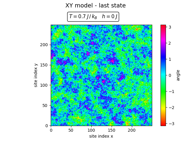
At low temperature one still sees large correlated regions, even though in the thermodynamic limit true long-range order is absent. Because the lattice in the simulation is finite, the system can effectively select one global orientation and fluctuate only weakly around it. This behaviour is related to the finite-size effects discussed earlier: although long-wavelength spin waves prevent true spontaneous symmetry breaking in the thermodynamic limit, on a finite lattice the system may still appear magnetised for long periods of time.
The same finite-size effects also affect the Monte Carlo sampling. As mentioned earlier in the discussion of the Metropolis algorithm, the assumption that the Markov chain efficiently explores the whole configuration space can become problematic at low temperatures. In practice the simulation may remain trapped near one orientation of the spins, which is why the low-temperature configuration above shows relatively small angular fluctuations.
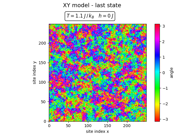
At high temperature the configuration is visibly more disordered.
The video illustrates the same physics more directly: vortices and antivortices appear as localized defects in the spin field, and at low temperatures they tend to remain pairwise bound.
Results and discussion
A particularly clear quantity is the autocorrelation time. The two plots below show the autocorrelation function at \(T=0.7\) and \(T=1.1\) for \(h=0\).
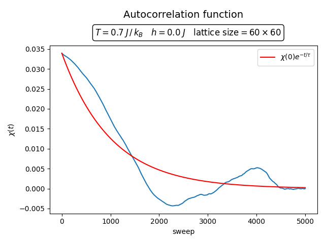
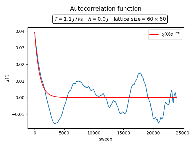
If the temperature is high, the autocorrelation function follows the exponential approximation quite accurately, at least in the initial regime where \(\chi(t)>0\). At low temperatures the decay is slower and the difference between the exponential fit and the actual values becomes significant. This supports the concern already mentioned above: at low temperatures the finite lattice may fail to explore configuration space properly and can get stuck around a non-zero magnetisation.
The corresponding autocorrelation times are shown below.
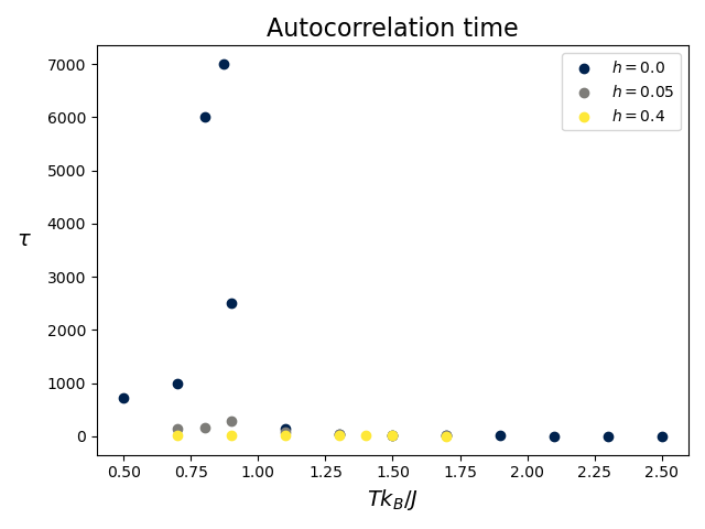
Without an external magnetic field, one can clearly see the existence of a critical point around \(T_C \approx 0.9\). The autocorrelation time grows strongly there, as expected from the Kosterlitz–Thouless transition theory. At low temperatures the autocorrelation time is not properly defined and its value differs between runs. This again arises from the finite-size effects already discussed.
The same figure also displays the effect of external magnetic fields. Even in the case of a weak field \(h=0.05\), the autocorrelation time no longer diverges at the critical point. Although the values are still somewhat larger at low temperatures, they remain in a reasonable range. A stronger magnetic field \(h=0.4\) decreases the autocorrelation time dramatically. This supports the main message of the simulation: the external magnetic field effectively removes the topological phase transition, although some critical behaviour remains.
The vortex-pair distance distributions tell a similar story.
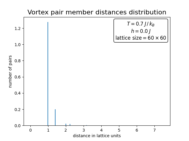
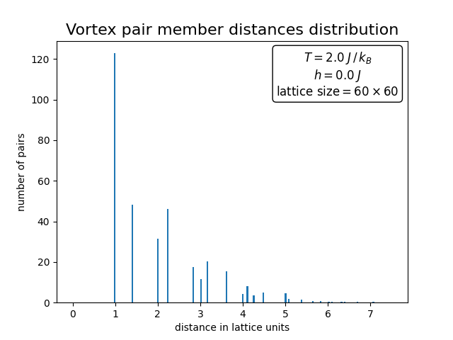
At low temperature there are relatively few vortices and they are mostly pairwise bound, with distances typically of one lattice spacing. At high temperature the distribution becomes much broader, signalling the unbinding of vortex pairs. This is one of the clearest geometric manifestations of the Kosterlitz–Thouless transition.
The simulation therefore reproduces the basic theoretical picture rather well. Without external magnetic field the model undergoes a topological phase transition associated with vortex unbinding and critical slowing down. When a magnetic field is applied, the transition disappears because the global \(U(1)\) symmetry is broken explicitly, but the system still exhibits some residual critical-looking behaviour.
Conclusion
What I find especially attractive about this project is that it makes a rather subtle phase transition visible in a very concrete way. The two-dimensional XY model does not fit the usual symmetry-breaking paradigm, yet it still exhibits non-trivial thermodynamic behaviour governed by topological defects. The simulation captures this picture quite well: one sees critical slowing down, vortex proliferation above the critical region, and the qualitative disappearance of the transition once an external magnetic field is applied.
1: J. Masák, E. Tõkke, Computational Physics Project 2: Monte Carlo simulation of the two-dimensional XY model, Course Project Report, Science faculty, Leiden university (2025), PDF.
2: N. D. Mermin, H. Wagner, Absence of ferromagnetism or antiferromagnetism in one- or two-dimensional isotropic Heisenberg models, Phys. Rev. Lett. 17 (1966) 1133, doi:10.1103/PhysRevLett.17.1133.
3: J. M. Kosterlitz, D. J. Thouless, Ordering, Metastability and Phase Transitions in Two-Dimensional Systems, J. Phys. C: Solid State Phys. 6 (1973) 1181, doi:10.1088/0022-3719/6/7/010.
4: N. Metropolis, A. W. Rosenbluth, M. N. Rosenbluth, A. H. Teller, E. Teller, Equation of State Calculations by Fast Computing Machines, J. Chem. Phys. 21 (1953) 1087, doi:10.1063/1.1699114.
5: J. Tobochnik, G. V. Chester, Monte Carlo Study of the Planar Spin Model, Phys. Rev. B 20 (1979) 3761, doi:10.1103/PhysRevB.20.3761.